
Excel Tutorial Summary: Freeze Rows and Columns in Excel
Learning how to freeze rows and columns in Excel is up there on the list of things you need to learn as an Excel newbie. This simple yet powerful feature allows you to scroll through large data sets, freeze dashboards, charts or pretty much any object in Excel by freezing rows or columns. Freezing rows and columns is especially helpful when you have information / data outside the cells that are displayed on your screen.
You can either watch the video located below or you can work through the step by step processes also located below..
Skill Level: Beginner
Table of Contents – How to Freeze Columns and Rows in Excel
1 – Video: How to Freeze Rows and Columns in Excel
2 – How to Freeze Rows in Excel
3- How to Freeze Columns in Excel
4 – How to Freeze Rows and Columns in Excel
Video: How to Freeze Rows & Columns in Excel

I’m a huge advocate for learning by video so in this clip, I’ll introduce and show you how to freeze rows and columns in Excel.
This section is made specifically for those of you who learn better by seeing / watching.
How to Freeze Rows in Excel
1
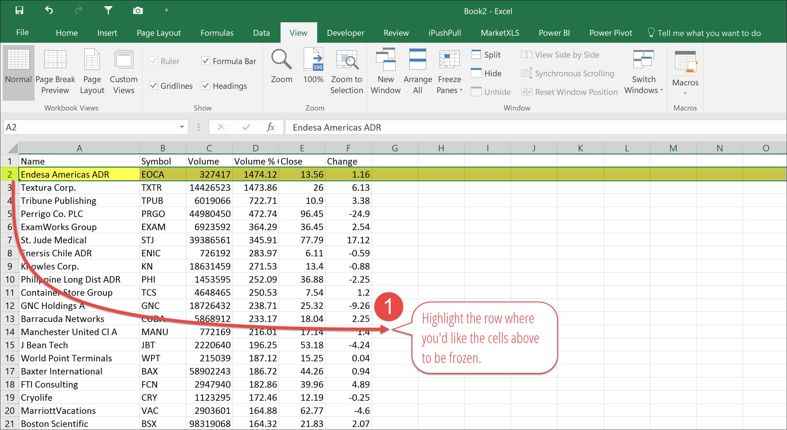
Select a Row
The first step of the process is to select the row (by highlighting the row number on the left). Any content/cells above the highlighted row will be frozen so that when you scroll through your worksheet, you’ll continue to see that content.
2
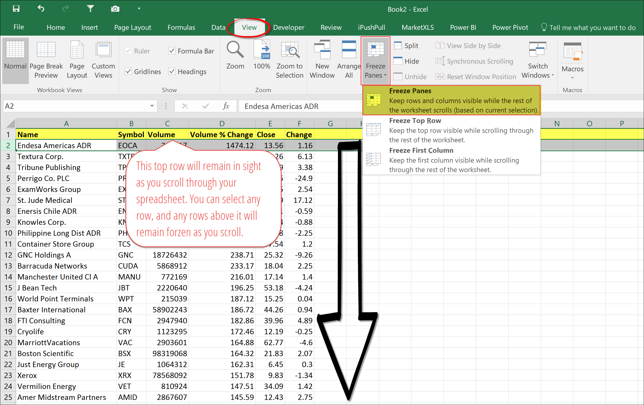
Select View & Freeze Panes
The second and last step of being able to freeze rows in Excel is to head over to the view tab of the quick access ribbon and select freeze panes. Once you’ve done this, as you scroll down through your spreadsheet, any rows above the row select will remain in sight on your worksheet.
How to Freeze Columns in Excel
1
Select a Column
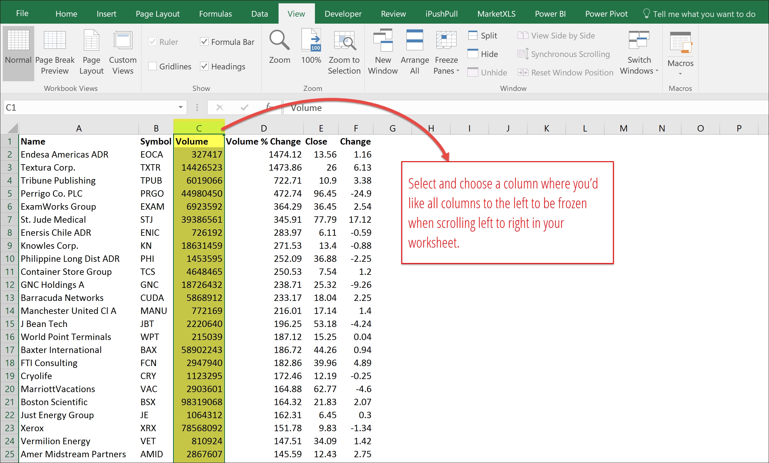
The first step of the process is to select the column (by highlighting the column letter on the top of your spreadsheet). Any content/cells left of the highlighted column will be frozen so that when you scroll through your worksheet from right to left, you’ll continue to see that content.
In the example below, I’ve frozen all columns to the left of column C so that we can see the stock name and its ticker symbol.
2
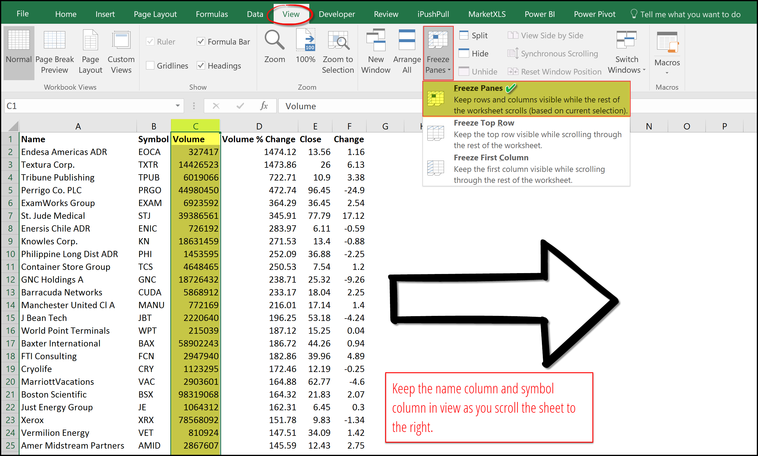
Select View & Freeze Panes to Freeze Columns
The second and last step of being able to freeze columns in Excel is to head over to the view tab of the quick access ribbon and select freeze panes. Once you’ve done this, as you scroll to the right in your spreadsheet, any columns to the left of your highlighted column will remain in sight on your worksheet.
How to Freeze Rows & Columns in Excel
1
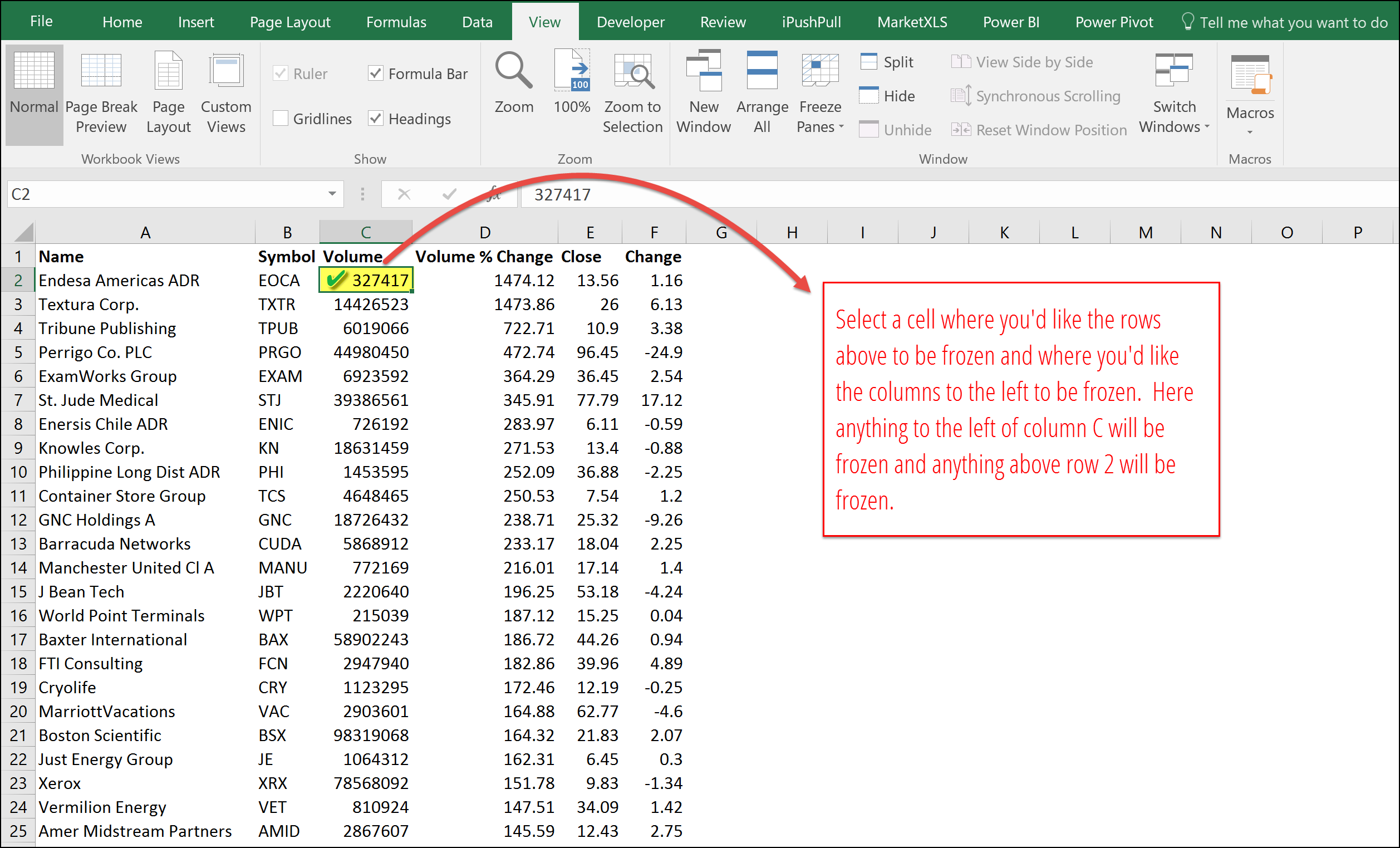
Select a Cell
The first step of the process is to select a cell whereby you want all columns to the left to be frozen and all rows above the cell to be frozen. This will then allow columns and rows to the left and above to always be shown when scrolling through your worksheet.
In the example below, I’ve selected cell C2 so that all columns to the left of column C and all rows above row 2 will remain frozen when scrolling.
2
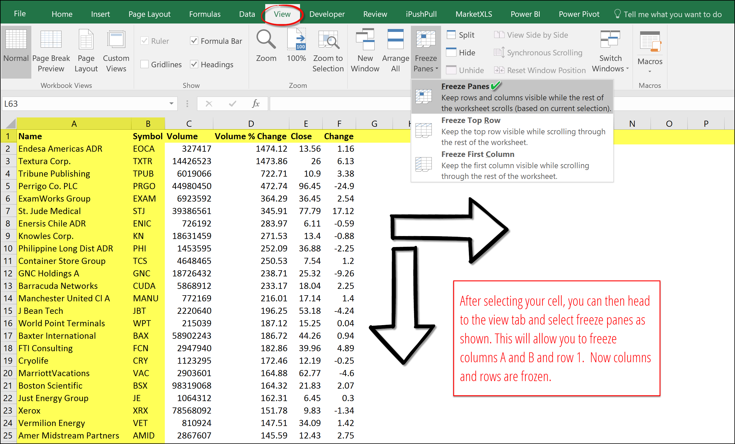
Select View & Freeze Panes to Freeze Columns and Rows
The second and last step of being able to freeze columns and rows at once in Excel is to head over to the view tab of the quick access ribbon and select freeze panes. Once you’ve done this, as you scroll to the right or down in your spreadsheet, any columns to the left and any rows above your highlighted cell will remain in sight on your worksheet.
Learn By Doing – Buy a $5 Dashboard


yeah! that is an essential thing for Excel!
Nice Article, thanks for sharing, Keep up the good work!
Great article, Thanks for sharing, keep up the good work!